
Notes
All years referred to in this report are calendar years. Numbers in the text, tables, and figures may not add up to totals because of rounding.
Under current law, the growth of federal noninterest spending and net outlays for interest on federal debt would outpace the increase in revenues over the next 30 years, the Congressional Budget Office projects. As a percentage of gross domestic product (GDP), federal debt held by the public is thus projected to climb from 102 percent at the end of 2021 to 202 percent in 2051.1 A perpetually rising debt-to-GDP ratio is unsustainable over the long term because financing deficits and servicing the debt would consume an ever-growing proportion of the nation’s income.
In this report, CBO analyzes the effects of measures that policymakers could take to prevent debt as a percentage of GDP from continuing to climb.2 Policymakers could restrain the growth of spending, raise revenues, or pursue some combination of those two approaches. Regardless of which method they chose, the policy change—and the timing of it—would directly affect the economy and the well-being of people.
Waiting to put fiscal policy on a sustainable course and allowing federal debt to continue to climb would have several effects on the economy. As federal borrowing increased, the amount of funds available for private investment would decline (a phenomenon known as crowding out), and interest costs would increase. Perpetually rising debt would also increase the likelihood of a fiscal crisis and pose other risks to the U.S. economy.
Many policy options are available to policymakers to stabilize debt as a percentage of GDP; for this analysis, CBO examined two simplified policies. The first would raise federal tax rates on different types of income proportionally. The second would cut spending for certain government benefit programs—mostly for Social Security, Medicare, and Medicaid. Under each of the two stylized policy options, debt as a percentage of GDP would be fully stabilized 10 years after the changes were implemented. CBO analyzed the effects of implementing the two options in three different years—2026, 2031, and 2036. To assess the effects of waiting to stabilize the debt 5 or 10 years, the agency calculated the differences in the estimated effects of implementing the policy changes in the two later years and implementing them in 2026.
CBO’s analysis yielded the following key findings:
- Regardless of when the process was begun, stabilizing federal debt as a percentage of GDP would require that income tax receipts or benefit payments change substantially from their currently projected path.
- The longer policymakers waited to implement a policy change, the more debt would grow in relation to GDP, and the greater the policy changes needed to stabilize it would be.
- If the option of increasing income tax rates was chosen, the effects of delaying implementation would be greater than they would be under the option of cutting benefits: Increases in interest costs would be larger, GDP and household consumption would be lower, and debt as a percentage of GDP would be higher in the long run.
- Under either option, the negative effects of delaying the implementation of policy changes on people’s consumption and labor supply would be disproportionately borne by younger people and lower-income people.
The Consequences of Rising Federal Debt
The high and rising federal debt that CBO projects over the next three decades would have serious consequences for the economy and federal budget, including the crowding out of private investment, higher interest costs, and increased risks of a fiscal crisis and of other disruptions.
Crowding Out of Private Investment
Increased government borrowing would, in CBO’s assessment, crowd out private investment in productive capital because the portion of private savings used to buy Treasury securities would no longer be available to fund such investment. When the government borrows, it does so from people and businesses whose savings would otherwise finance private investment in productive capital, such as factories and computers. An increase in government borrowing strengthens the incentive to save—in part, by driving up interest rates—but the increase in private saving is not as large as the increase in government borrowing; national saving, or the amount of domestic resources available for private investment, therefore declines.3 Private investment falls less than national saving does in response to government deficits because the higher interest rates that are likely to result from increased federal borrowing tend to attract more foreign capital into the United States. The decline in private investment reduces the capital stock below what it would be otherwise, which in turn reduces output.
If investment in capital goods declined, workers would, on average, have less capital to use in their jobs. As a result, they would be less productive, their compensation would be lower, and they would thus be less inclined to work. In turn, they would consume fewer goods and services. Those effects would increase over time as federal borrowing grew.
Rising Interest Costs
The projected increase in federal borrowing would also put upward pressure on interest rates, increasing the total burden of interest outlays on the federal budget.4 That effect would grow over time as the existing stock of outstanding debt matured and was rolled over into new Treasury securities with higher interest rates. Moreover, the federal budget would be more vulnerable to increases in interest rates because costs to service that debt rise more for a given increase in interest rates when debt is higher than when it is lower. Interest payments to foreign holders of U.S. debt would also increase as interest costs rose.
Risk of a Fiscal Crisis
The likelihood of a fiscal crisis increases as federal debt continues to rise in relation to GDP, because mounting federal debt could erode investors’ confidence in the government’s fiscal position and result in a sharp reduction in their valuation of Treasury securities. In turn, investors would demand higher yields to purchase Treasury securities and thus drive up interest rates on federal debt. Additionally, concerns about the U.S. government’s fiscal position could lead to a sudden increase in inflation expectations, fear of a large decrease in the value of the U.S. dollar, or a loss of confidence in the federal government’s ability to repay its debt in full, all of which would make a fiscal crisis more likely. If a fiscal crisis occurred, it would result from multiple factors, and no clear basis exists for identifying the level of debt that might lead to such a crisis in the United States.
Several characteristics of the U.S. financial system make a fiscal crisis less likely in the United States than in other countries, and financial markets do not currently reflect any notable concern about the risk of such a crisis in the United States. But given the persistently large budget deficits that are projected under current law and the already high debt-to-GDP ratio, the risk of a fiscal crisis is likely to be higher in the future if steps are not taken to stabilize the debt.
Risk of Other Disruptions
Even in the absence of an abrupt fiscal crisis, high and rising debt could have persistent negative effects on the economy beyond those incorporated in CBO’s extended baseline projections, including a gradual decline in the value of Treasury securities and other domestic assets. Debt’s current trajectory could cause people’s inflation expectations to rise moderately but persistently. Increases in federal borrowing could also lead to an erosion of confidence in the U.S. dollar as the world’s dominant currency. Such developments would make it more difficult to finance public and private activity. Moreover, the increased dependence on foreign investors that would accompany high and rising debt could pose other challenges, such as making U.S. financial markets more vulnerable to a change in the valuation of U.S. assets by participants in global markets. High and rising debt might also cause policymakers to feel constrained from implementing deficit-financed fiscal policy to respond to unforeseen events or for other purposes, such as to promote economic activity or strengthen national defense.
Two Illustrative Options for Stabilizing Debt
The effects of waiting to address the long-term budget imbalance would depend on the policy changes that were adopted to put the government’s finances on a sustainable path and the timing of those policy changes. CBO examined the economic effects of two illustrative policy options:
- Gradually Increase Personal Income Tax Rates. Personal income tax rates on labor income and on capital income would increase over time in proportion to the rates that were in effect in 2021. The increases would not alter the progressivity of the tax system because both marginal and average tax rates would increase proportionally for all income levels.
- Gradually Cut Benefit Payments. Under this option, Social Security benefits and spending for the government’s major health care programs would be cut proportionally to each program’s share of total government spending.5
Those stylized policies were chosen as simple examples to illustrate the economic effects of stabilizing debt as a percentage of GDP at different points in the future.6 Policies that combined tax increases with benefit cuts would result in outcomes that were somewhere between those estimated under the two stylized options.
CBO’s Methods for Estimating the Effects of Waiting to Stabilize the Debt
CBO analyzed the effects of implementing the two stylized policy options in 2026, 2031, and 2036. In all six scenarios, the policies would stabilize debt as a percentage of GDP over a 10-year period, but the level at which debt would be stabilized under each scenario varies widely. The agency’s estimates incorporate the economic effects of changes to revenues and spending and how those economic changes would, in turn, affect the budget; that is, they incorporate the effects of what is often referred to as budgetary feedback.
In each of the six illustrative scenarios that CBO simulated, the policy change is announced immediately, and people begin to adjust their behavior accordingly. They therefore have more time to adjust their behavior the later the changes are scheduled to take effect.
CBO estimated the effects that the delayed start dates would have on the overall economy and on the economic well-being of people of different generations and in different income groups. To quantify the effects on the economy, CBO estimated the effects on the capital stock, the labor supply, output, and total consumption. To quantify the effects on people’s economic well-being, the agency examined two measures—lifetime consumption and lifetime hours worked. CBO estimated the effects of a 5-year delay by calculating the difference between outcomes under the scenarios in which each policy option is implemented in 2031 and those under the scenarios in which it is implemented in 2026; for the 10-year delays, the agency compared outcomes under the scenarios in which the options take effect in 2036 with those under the scenarios in which they take effect in 2026.
CBO first estimated the changes in budgetary and economic outcomes under each of the six illustrative scenarios in relation to a benchmark scenario in which debt is not stabilized. To make the analysis tractable, the agency used a benchmark that is a simplified version of the extended baseline projections that CBO published in March 2021. The agency simplified those baseline projections by excluding short-term cyclical factors, such as those occurring in 2022 in the wake of the coronavirus pandemic. As a result, the budget and economic projections for 2022 in this analysis look more like the baseline in 2031—when short-term cyclical factors are absent—than the baseline in 2022. In the benchmark scenario, federal spending for benefit payments in 2021 measured as a share of GDP equals the average of such spending over the 2021–2051 period in the extended baseline projections.
The focus on the long term mostly affects the total budgetary amounts—total revenues, spending, and debt—presented in this report. For example, debt as a percentage of GDP is a few percentage points higher in 2022 in the benchmark than it is in CBO’s extended baseline projections. The effects of the policies—that is, the difference between outcomes under any one of the policy options considered in this report and the benchmark—would differ by only small amounts if the agency’s baseline projections had been used as the benchmark.
Effects That Waiting to Stabilize the Debt Would Have on the Economy
In the benchmark economy used in this analysis—an economy in which no stabilization policy is enacted—income tax revenues and benefit payments rise over the 2021–2051 period and peak at 10.3 percent of GDP and 14.5 percent of GDP, respectively. If stabilization began in 2026, income tax revenues would rise as high as 11.9 percent of GDP and benefit payments would fall as low as 11.1 percent of GDP by 2035.
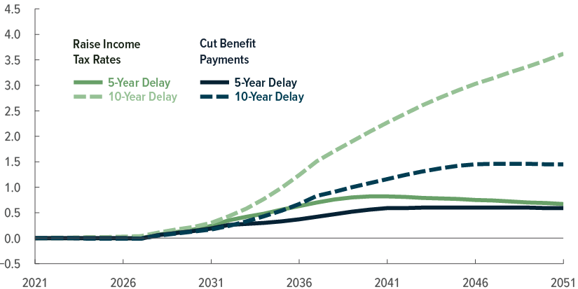
The change in income tax revenues or benefit payments needed to stabilize the debt would be greater if stabilization was delayed. For example, if stabilization through increases in tax rates was delayed by 5 years and began in 2031, income tax revenues would, at their highest point, need to be 0.8 percent of GDP higher than they would be if the process was begun in 2026; a 10-year delay would require revenues that were 3.7 percent of GDP higher at their peak than they would be with no delay (see Figure 1). Alternatively, if stabilization through reductions in benefit payments was delayed by 5 years, those payments would, at their lowest point, need to be 0.4 percent of GDP lower than they would be without a delay; a 10-year delay would require benefit payments that were 0.9 percent of GDP lower at their trough.
Figure 1.
Tax Revenues and Benefit Payments Under Two Options for Stabilizing Federal Debt Starting in Three Different Years
Percentage of GDP
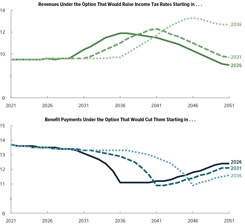
The longer stabilization was delayed, the higher income tax revenues—and thus income tax rates—would ultimately need to be to stabilize federal debt as a percentage of GDP.
Likewise, the cuts in benefit payments would, in the long run, need to be greater the longer stabilization was delayed.
Data source: Congressional Budget Office. See www.cbo.gov/publication/57867#data.
Under the first illustrative option, personal income tax rates on labor income and on capital income would gradually increase over time in proportion to the rates under current law. Under the second, Social Security benefits and spending for the government’s major health care programs (namely, outlays for Medicare, Medicaid, and the Children’s Health Insurance Program and subsidies for health insurance purchased through the marketplaces established under the Affordable Care Act or through the Basic Health Program) would gradually be cut in proportion to each program’s share of total government spending under current law. In all the simulated scenarios, the policy change is announced immediately, so people have more time to adjust their behavior the later the change is scheduled to take effect. Debt would be fully stabilized as a percentage of GDP 10 years after the policy change went into effect.
In all the simulated scenarios, the changes in revenues or benefit payments are smaller for the first few years after stabilization begins than they are later on because the policy changes are phased in over 10 years. The increases in revenues or decreases in benefit payments are particularly small from 2026 to 2030 in the scenarios in which debt stabilization begins in 2026 because, under current law, deficits in those years are projected to be smaller than deficits in 2031 and beyond.
GDP = gross domestic product.
Regardless of the policy option used to stabilize the debt, debt as a percentage of GDP—and thus the level at which debt would ultimately be stabilized—would rise the longer the process was delayed; however, if stabilization was achieved by raising income taxes, the debt-to-GDP ratio would reach higher levels than it would if benefit payments were cut (see Figure 2). That is at least in part because GDP would be lower after an increase in income tax rates than it would be after cuts in benefit payments (see Figure 3). Whereas benefit cuts strengthen people’s incentives to work and save, tax increases weaken those incentives and thus reduce the capital stock, the labor supply, and output. Moreover, if tax increases were used to stabilize debt, delaying implementation of those increases would have a much larger effect on after-tax wages and returns on capital than delaying benefit cuts would. Both policies would affect people of different generations and of different income levels to varying degrees.
Figure 2.
Federal Debt Under Two Options for Stabilizing It Starting in Three Different Years
Percentage of GDP

Debt would continue to rise as a percentage of GDP even after policy changes were implemented, so the longer stabilization was delayed, the higher the level debt would ultimately reach. In addition, debt would stabilize at a higher level under the option that would raise income tax rates than it would under the option that would cut benefit payments, all else being equal.
Data source: Congressional Budget Office. See www.cbo.gov/publication/57867#data.
Under the first illustrative option, personal income tax rates on labor income and on capital income would gradually increase over time in proportion to the rates under current law. Under the second, Social Security benefits and spending for the government’s major health care programs (namely, outlays for Medicare, Medicaid, and the Children’s Health Insurance Program and subsidies for health insurance purchased through the marketplaces established under the Affordable Care Act or through the Basic Health Program) would gradually be cut in proportion to each program’s share of total government spending under current law. In all the simulated scenarios, the policy change is announced immediately, so people have more time to adjust their behavior the later the change is scheduled to take effect. Debt would be fully stabilized as a percentage of GDP 10 years after the policy change went into effect.
GDP = gross domestic product.
Figure 3.
Effects That Delaying Two Options for Stabilizing Federal Debt Would Have on GDP
Percent

If stabilization was achieved by increasing income tax rates, delaying implementation by 5 or 10 years would have only a small effect on GDP through 2036 but would lower GDP more thereafter. By contrast, if benefit payments were cut, delaying stabilization would increase GDP through 2051 and beyond, though the effect would be minimal.
Data source: Congressional Budget Office. See www.cbo.gov/publication/57867#data.
Under the first illustrative option, personal income tax rates on labor income and on capital income would gradually increase over time in proportion to the rates under current law. Under the second, Social Security benefits and spending for the government’s major health care programs (namely, outlays for Medicare, Medicaid, and the Children’s Health Insurance Program and subsidies for health insurance purchased through the marketplaces established under the Affordable Care Act or through the Basic Health Program) would gradually be cut in proportion to each program’s share of total government spending under current law. In all the simulated scenarios, the policy change is announced immediately, so people have more time to adjust their behavior the later the change is scheduled to take effect. Debt would be fully stabilized as a percentage of GDP 10 years after the policy change went into effect.
To estimate the effects of a 5-year delay, CBO calculated the difference between outcomes under scenarios in which each policy change would go into effect in 2031 and those under scenarios in which it would take effect in 2026; for the 10-year delays, the agency compared outcomes under scenarios in which the change would take effect in 2036 with those under scenarios in which it was implemented in 2026. A positive value indicates an increase, and a negative value, a decrease.
GDP = gross domestic product.
Stabilization Through Increases in Income Tax Rates
Most of the long-term economic effects of delaying stabilization through increases in tax rates would stem from the crowding-out effects of higher deficits and debt on the capital stock. Additionally, the higher tax rates that would be required if implementation of the policy was delayed would reduce after-tax wages, which would discourage work and lower the aggregate supply of labor. Those reductions in capital stock and the labor supply would cause GDP to be lower than it would be if the policy was implemented earlier, which, in turn, would necessitate an even larger increase in tax rates to stabilize debt as a percentage of GDP.
A delay of 5 or 10 years in increasing tax rates would crowd out investment and reduce the size of the capital stock in 2051 by about 1.5 percent and 4.0 percent, respectively (see Table 1). Delays in implementing such a policy would also reduce the labor supply in 2051—a 5-year delay, by 0.4 percent, and a 10-year delay, by 1.7 percent. The labor supply would be reduced in the long run because some people would choose to work fewer hours for two reasons. First, delaying action would require a larger increase in income tax rates to stabilize debt as a percentage of GDP, and those higher rates would weaken the incentive to work more than would the rate increases that would be necessary if the policy was implemented earlier. Second, a smaller capital stock implies lower before-tax wages, which would further weaken the incentive to work. As a result, GDP would be 0.9 percent lower in 2051 if implementation of the policy was delayed by 5 years and 2.6 percent lower if it was delayed by 10 years. The decline in total consumption would be smaller in percentage terms than the decline in GDP because the reduced capital stock resulting from a delay would lower both the saving rate and the amount of depreciation.
Table 1.
Effects That Delaying Two Options for Stabilizing Federal Debt Would Have on Macroeconomic Variables in 2051
Percent

Data source: Congressional Budget Office. See www.cbo.gov/publication/57867#data.
Under the first illustrative option, personal income tax rates on labor income and on capital income would gradually increase over time in proportion to the rates under current law. Under the second, Social Security benefits and spending for the government’s major health care programs (namely, outlays for Medicare, Medicaid, and the Children’s Health Insurance Program and subsidies for health insurance purchased through the marketplaces established under the Affordable Care Act or through the Basic Health Program) would gradually be cut in proportion to each program’s share of total government spending under current law. In all the simulated scenarios, the policy change is announced immediately, so people have more time to adjust their behavior the later the change is scheduled to take effect. Debt would be fully stabilized as a percentage of GDP 10 years after the policy change went into effect.
To estimate the effects of a 5-year delay, CBO calculated the difference between outcomes under scenarios in which each policy change would go into effect in 2031 and those under scenarios in which it would take effect in 2026; for the 10-year delays, the agency compared outcomes under scenarios in which the change would take effect in 2036 with those under scenarios in which it was implemented in 2026. A positive value indicates an increase, and a negative value, a decrease.
GDP = gross domestic product; * = between zero and 0.05 percent; ** = between zero and 0.05 percentage points.
As a percentage of GDP, federal net interest costs would increase the longer stabilization was delayed (see Figure 4). That increase would occur because debt would continue to grow—and the interest rate on it would continue to rise—the longer implementation of the policy was delayed.
Figure 4.
Effects That Delaying Two Options for Stabilizing Federal Debt Would Have on Net Interest Costs
Percentage of GDP
Data source: Congressional Budget Office. See www.cbo.gov/publication/57867#data.
Under the first illustrative option, personal income tax rates on labor income and on capital income would gradually increase over time in proportion to the rates under current law. Under the second, Social Security benefits and spending for the government’s major health care programs (namely, outlays for Medicare, Medicaid, and the Children’s Health Insurance Program and subsidies for health insurance purchased through the marketplaces established under the Affordable Care Act or through the Basic Health Program) would gradually be cut in proportion to each program’s share of total government spending under current law. In all the simulated scenarios, the policy change is announced immediately, so people have more time to adjust their behavior the later the change is scheduled to take effect. Debt would be fully stabilized as a percentage of GDP 10 years after the policy change went into effect.
To estimate the effects of a 5-year delay, CBO calculated the difference between outcomes under scenarios in which each policy change would go into effect in 2031 and those under scenarios in which it would take effect in 2026; for the 10-year delays, the agency compared outcomes under scenarios in which the change would take effect in 2036 with those under scenarios in which it was implemented in 2026. A positive value indicates an increase, and a negative value, a decrease.
GDP = gross domestic product.
Stabilization Through Reductions in Benefit Payments
Stabilizing debt as a percentage of GDP by reducing benefit payments would affect the economy through two primary channels. First, a drop in benefits would reduce people’s income and induce some people to work more to, at least partially, maintain their standard of living, thereby increasing the aggregate labor supply. Second, a drop in expected future retirement benefits would induce workers to save more before they retired, and that increased saving would, in turn, increase the aggregate capital stock.
A 5-year delay in implementing such a policy would lower the size of the capital stock in 2051 by 0.1 percent and increase the labor supply by 0.2 percent. That year, GDP would be 0.1 percent higher than it would be without the delay, and total consumption would be 0.1 percent lower.
If the cuts were delayed by 10 years, the capital stock in 2051 would be unaffected, and the labor supply would increase by 0.4 percent. The increase in the labor supply would result in GDP that was 0.2 percent higher and total consumption that was 0.2 percent lower that year than they would be if implementation of the policy was not delayed.
Effects That Waiting Would Have on People of Different Generations and Income Levels
To analyze how delaying stabilization under the two policies would affect people of different generations and income levels, CBO first divided the population into 20-year birth cohorts and then divided each cohort into thirds on the basis of people’s labor income.
To quantify and compare the effects of waiting to stabilize federal debt on different people, CBO focused on lifetime consumption and lifetime hours worked. Changes in those two measures vary among people within the same generation for a variety of reasons, so CBO computed the averages for each generation and for each of the three income groups within the generations.
Comparing the change in consumption among generations provides only a partial picture of their comparative well-being. Technological advancement leads to a steadily increasing level of consumption per capita over time, so later generations enjoy higher standards of living over their lifetimes. Although delaying debt stabilization would reduce future generations’ lifetime consumption, those generations would probably remain better off in absolute terms than earlier generations because their absolute level of consumption would be much higher.
Stabilization Through Increases in Income Tax Rates
If the policy of increasing tax rates was used to stabilize debt, delaying stabilization would increase the consumption of older cohorts and lower that of younger ones. Because many older people would have retired, they would be affected primarily by the change in the tax rate on capital income, which would be smaller than the change in the rate on labor income. Moreover, the increases in taxes on their savings would be offset by increases in the interest they earned on that savings. By contrast, younger people would face higher taxes on their labor income.
People born between 1940 and 1979 would see an increase in lifetime consumption ranging from 0.1 percent to 0.4 percent if stabilization was delayed by 5 years (see Table 2). The percentage increase would be slightly larger for people in the bottom third of the income distribution in those cohorts because the tax policy used to stabilize debt is progressive—lower-income people’s effective tax rates would increase by less than higher-income people’s rates would.7 A 10-year delay in implementation would increase those cohorts’ consumption by between 0.2 percent and 0.9 percent because the increases in the effective tax rates would be larger than they would be with a 5-year delay.
Table 2.
Effects That Delaying Two Options for Stabilizing Federal Debt Would Have on Consumption Over People’s Lifetime, by Birth Cohort and Income Group
Percent

Data source: Congressional Budget Office. See www.cbo.gov/publication/57867#data.
Under the first illustrative option, personal income tax rates on labor income and on capital income would gradually increase over time in proportion to the rates under current law. Under the second, Social Security benefits and spending for the government’s major health care programs (namely, outlays for Medicare, Medicaid, and the Children’s Health Insurance Program and subsidies for health insurance purchased through the marketplaces established under the Affordable Care Act or through the Basic Health Program) would gradually be cut in proportion to each program’s share of total government spending under current law. In all the simulated scenarios, the policy change is announced immediately, so people have more time to adjust their behavior the later the change is scheduled to take effect. Debt would be fully stabilized as a percentage of gross domestic product 10 years after the policy change went into effect.
To estimate the effects of a 5-year delay, CBO calculated the difference between outcomes under scenarios in which each policy change would go into effect in 2031 and those under scenarios in which it would take effect in 2026; for the 10-year delays, the agency compared outcomes under scenarios in which the change would take effect in 2036 with those under scenarios in which it was implemented in 2026. A positive value indicates an increase, and a negative value, a decrease.
* = between zero and 0.05 percent.
For the cohort born between 1980 and 1999, people in the bottom third of the income distribution would consume slightly more if implementation of the policy was delayed by 5 years than they would if there was no delay, but the two-thirds of that cohort with higher income would consume slightly less with such a delay. If the policy change was delayed by 10 years, lifetime consumption would, on average, rise for people in the cohort regardless of their income. That effect is driven by the older members of the cohort, who either would have retired or would be near retirement by the time the policy change took effect in 2036 and whose exposure to the higher tax rates would thus be limited. The increase in consumption would be greatest for the bottom third of the income distribution in the cohort.
The cohort of people born after 1999 would be most affected by a 5-year delay. The consumption of all income groups in that cohort would fall; the highest-income people would experience the greatest declines. Delaying stabilization an additional 5 years would increase all those losses.
Delaying stabilization would also reduce the average number of hours people in most cohorts worked over their lifetime (see Table 3). Only the lifetime hours worked of people in the oldest cohort—those born between 1940 and 1959—would be largely unaffected: Most of those people will retire by 2026, and whether the increase in tax rates took effect that year or later would thus have little bearing on their behavior.
Table 3.
Effects That Delaying Two Options for Stabilizing Federal Debt Would Have on Hours Worked Over People’s Lifetime, by Birth Cohort and Income Group
Percent

Data source: Congressional Budget Office. See www.cbo.gov/publication/57867#data.
Under the first illustrative option, personal income tax rates on labor income and on capital income would gradually increase over time in proportion to the rates under current law. Under the second, Social Security benefits and spending for the government’s major health care programs (namely, outlays for Medicare, Medicaid, and the Children’s Health Insurance Program and subsidies for health insurance purchased through the marketplaces established under the Affordable Care Act or through the Basic Health Program) would gradually be cut in proportion to each program’s share of total government spending under current law. In all the simulated scenarios, the policy change is announced immediately, so people have more time to adjust their behavior the later the change is scheduled to take effect. Debt would be fully stabilized as a percentage of gross domestic product 10 years after the policy change went into effect.
To estimate the effects of a 5-year delay, CBO calculated the difference between outcomes under scenarios in which each policy change would go into effect in 2031 and those under scenarios in which it would take effect in 2026; for the 10-year delays, the agency compared outcomes under scenarios in which the change would take effect in 2036 with those under scenarios in which it was implemented in 2026. A positive value indicates an increase, and a negative value, a decrease.
* = between -0.05 percent and 0.05 percent.
Lifetime hours worked for all other cohorts would decline by between 0.1 percent and 0.7 percent. The reductions would be greater for younger cohorts than for older ones because a larger portion of the working life of people in those cohorts would occur during the period in which tax rates were higher. The differences in lifetime hours worked among income groups within the same cohort would be small.
Stabilization Through Reductions in Benefit Payments
If reductions in benefit payments were used to stabilize debt, delaying implementation of the policy would increase the consumption of higher-income groups and reduce that of the lowest-income group in most cohorts. As is the case under the policy affecting taxes, lifetime consumption among people born before 1980 would increase, on average, the longer it took to implement the policy. Delaying implementation would enable those people to receive their retiree benefit payments at the higher rate for longer before the reductions occurred.
For the two birth cohorts comprising people born since 1980, lifetime consumption would fall for people in the lowest third of the income distribution if implementation of the benefit was delayed by 5 years; the youngest people would experience the largest reductions. Benefits make up a larger proportion of the total lifetime resources of people with lower income, so the loss of benefits is not offset by the additional income they would earn from working more. Those two groups’ reductions in consumption would be larger if implementation of the policy change was instead delayed by 10 years.
By contrast, lifetime consumption of people in the top two-thirds of the income distribution in those age cohorts would generally be higher if implementation was delayed by 5 years because, in anticipation of the change, those people would work more to increase their earned income. For the top third of the income distribution in each of those cohorts, the increase in consumption would be larger the longer the delay in implementing the policy. The middle third of the income distribution in each of those cohorts would experience only small changes in consumption with the additional delay.
Delaying the implementation of benefit cuts would, on average, increase the number of hours people worked over their lifetime because an expected loss in benefits would induce people to work more to replace that lost income. The changes would be greater for younger people because the policy change would be in effect for a larger portion of their life. Only people in the bottom and middle thirds of the income distribution in the oldest cohort and people in the bottom third of the distribution in the second-oldest cohort would work slightly fewer hours if implementation of the policy was delayed. A delay would allow them to retire and receive larger benefit payments in the period before the cuts took effect, so they would not need to work as much to offset their lost retirement income. For all other people, the longer the delay, the more hours they would work over their lifetime, and the less time they would spend on other activities.
How CBO Modeled Behavioral Responses to Policy Changes
CBO analyzed the costs of delaying fiscal stabilization using its life-cycle model of the economy.8 In that model, people make decisions about how much to work and save on the basis of current economic conditions and government policies and their expectations about future conditions and policies. The analysis therefore reflects the way that people respond, on average, to changes in economic conditions and policies. For example, if the amount of income that people expected to receive in the future declined—because they expected their after-tax earnings to be lower than they had previously anticipated or because they expected cuts in their retirement benefit payments—they would work and save more in the meantime in anticipation of that loss.
Another notable feature of the model is that the increase in debt attributable to budget deficits, when everything else is held constant, causes the interest rate that the government pays on its debt to rise. That occurs, in CBO’s assessment, because greater federal borrowing ultimately crowds out private investment. When the stock of private capital is smaller, the value of each unit of available capital is driven up, increasing the return on that capital and the interest rate. In addition, the interest rate on government debt must rise as the risk of default goes up to induce people to hold a now riskier asset.
One last characteristic that should be noted is that the model uses a simplified representation of fiscal policy: For revenues, approximations of the progressive personal income tax, payroll taxes, and excise taxes were used; for expenditures, Social Security benefits, Medicare benefits, and a lump sum approximating payments for certain other benefit programs were used.
Limitations and Uncertainty
CBO’s estimates of the effects that delaying the implementation of policies to stabilize federal debt would have on the economy and on people’s well-being are highly uncertain because this analysis has some limitations. The estimates do not, for example, account for two key effects that delaying action would have: The government’s ability to respond to unexpected needs would be reduced, and the risk of a fiscal crisis would increase.
Moreover, the economy is subject to many contingencies, such as severe weather, changes in energy prices, and financial disturbances. Economic shocks that moved the economy into recession could have significant effects on the debt-to-GDP ratio and on other macroeconomic measures that are not reflected in this analysis. Also, the budget projections, which extend several decades into the future, are themselves uncertain, as are the estimates of the effects of changes in fiscal policy.
Another limitation is that the analysis reflects the way people have responded to policy changes in the past. Although past behavior is the best predictor available, people will not necessarily respond in the same way in the future.
1. Those estimates, which are part of what CBO calls its extended baseline projections, reflect economic conditions and the budgetary effects of laws enacted as of January 12, 2021. See Congressional Budget Office, The 2021 Long-Term Budget Outlook (March 2021), www.cbo.gov/publication/56977. CBO will update its extended baseline projections later in 2022.
2. In addition to the debt-to-GDP ratio used in this analysis, CBO regularly examines other measures of the long-term budget imbalance, including primary deficits and net interest costs.
3. In CBO’s assessment, another reason that an increase in government borrowing would strengthen the incentive to save is that some people would expect policymakers to raise taxes or cut spending in the future to cover the cost of paying interest on the additional federal debt. As a result, some of those people would increase their saving to prepare for paying higher taxes or receiving less in benefits. For further discussion of that effect and the estimated effect that changes in federal borrowing have on private investment, see Jonathan Huntley, The Long-Run Effects of Federal Budget Deficits on National Saving and Private Domestic Investment, Working Paper 2014-02 (Congressional Budget Office, February 2014), www.cbo.gov/publication/45140.
4. See Edward Gamber and John Seliski, The Effect of Government Debt on Interest Rates, Working Paper 2019-01 (Congressional Budget Office, March 2019), www.cbo.gov/publication/55018.
5. Spending for the major health care programs consists of outlays for Medicare, Medicaid, and the Children’s Health Insurance Program and subsidies for health insurance purchased through the marketplaces established under the Affordable Care Act or through the Basic Health Program.
6. Options to stabilize the federal debt could include increases in other types of taxes or reductions in other types of federal spending that are not addressed in this report. For more specific examples of such options, see Congressional Budget Office, Options for Reducing the Deficit: 2021 to 2030 (December 2020), www.cbo.gov/publication/56783.
7. Because income tax rates are progressive (that is, higher incomes are generally taxed at a higher rate than are lower incomes) and the option would increase rates proportionally, the rate increase would be smaller for people with lower income than it would be for those with higher income.
8. The model is an example of what is often called an overlapping generations model. For details about the model, see Congressional Budget Office, An Overview of CBO’s Life-Cycle Growth Model (February 2019), www.cbo.gov/publication/54985; and Shinichi Nishiyama, Fiscal Policy Effects in a Heterogeneous-Agent Overlapping-Generations Economy With an Aging Population, Working Paper 2013-07 (Congressional Budget Office, December 2013), www.cbo.gov/publication/44941.
This report supplements The 2021 Long-Term Budget Outlook, which is a part of a series of reports on the state of the budget and the economy that the Congressional Budget Office issues each year. In keeping with CBO’s mandate to provide objective, impartial analysis, this report makes no recommendations.
Kerk Phillips and Jaeger Nelson prepared the report with guidance from Devrim Demirel, John Kitchen, and Jeffrey Werling. Christina Hawley Anthony, John McClelland, and Andre Neveu (a visiting scholar at CBO) offered comments.
Mark Doms, Jeffrey Kling, and Robert Sunshine reviewed the report. Bo Peery edited it, and Jorge Salazar created the graphics and prepared the text for publication. The report is available at www.cbo.gov/publication/57867.
CBO seeks feedback to make its work as useful as possible. Please send comments to communications@cbo.gov.

Phillip L. Swagel
Director