Measuring the Cost of Government Activities That Involve Financial Risk

Many of the federal government’s activities involve financial risk, which can take various forms. For example, the government provides support for risky credit activities through investment and insurance programs. In addition, the government issues loans and guarantees loans made by private financial institutions, which expose it to the risk of high rates of default. It insures bank deposits and pension funds, which expose it to the risk of higher costs if many banks fail or if pension investments earn smaller returns than expected. The government levies taxes, which produce revenues that fluctuate depending on the performance of the economy. Likewise, spending automatically varies for the safety-net programs that the government provides, again depending on economic conditions. 

All of those activities create the risk that deficits will be larger than expected when the economy is weak, as well as the possibility that they will be smaller than expected when the economy is strong. That risk is passed on to government stakeholders—both beneficiaries of government programs and taxpayers—for whom, as investors, it would have a cost. An increased deficit in a weak economy occurs when resources are scarce and particularly valuable and incomes are low. Because people find costs to be particularly burdensome under those circumstances, positive and negative deviations from the average do not balance out when people weigh the risks associated with future outcomes.

One approach to measuring the cost of government activities uses their projected average budgetary effects. The estimated cost of most government activities, including those that are subject to risk, is based on their average projected effect on the government’s cash flows. For example, the Federal Credit Reform Act of 1990 (FCRA) bases the cost of loans and loan guarantees on their average default rates and the associated losses.

An alternative approach, called fair value, incorporates a fuller cost of risk than is reflected in the average budgetary effects. Fair value includes market risk, which is the financial risk that remains even with a well-diversified portfolio and that depends solely on the performance of the economy. Government stakeholders are exposed to that risk when the government provides credit assistance or invests in a financial asset, such as an ownership stake in a private business. The fair-value approach provides information to policymakers on the cost of such risk, whereas the FCRA approach does not.

Estimated costs can differ significantly depending on how they are measured—budget savings under FCRA can become costs under fair value, for instance—and those costs directly affect the federal budget and the resulting deficits and debt. This Congressional Budget Office report explains the details of each approach, the qualitative differences between them, and their application to various activities and programs.

The Current Budgetary Treatment of Federal Credit Programs

Costs of loans and loan guarantees are recorded up front as a present value—as required by FCRA—because the cash flows are spread out over time. (A present value is a single number that expresses the flow of current and future payments or income in terms of an equivalent lump sum paid or received at a specified time. A present value depends on the rate of interest, or discount rate, used to translate a cash flow in a future year into current dollars.) That method of accounting measures the costs of loans and loan guarantees on a comparable basis, though the timing of their cash flows is very different.

The present value is calculated using projections of future cash flows that reflect average rates of default and that are discounted to the present using the interest rates on Treasury securities (which represent the government’s cost of borrowing). The projected cash flows include any fees and interest payments that the government receives, which can offset the projected cost of defaults.

Comparisons of the costs of different types of credit programs are easier to make using FCRA estimates than using cash estimates because FCRA estimates show the projected cost of a loan or loan guarantee over its lifetime when it is made. In contrast, cash estimates only show costs over the 10-year period considered in the Congressional budget process, so they could give misleading information about the costs of credit programs that extend beyond that period. Estimated on a cash basis, the cost of direct loans could appear larger than the cost of guaranteed loans made to the same borrowers, for example, because the budget projection period would truncate the costs of the guarantees and the repayment of the direct loans when those loans and loan guarantees have payments that extend beyond 10 years. (The actual costs to the government of the loans and guarantees could be the same, but their cash flows would differ.)

Fair Value: An Alternative Approach That Reflects Market Risk

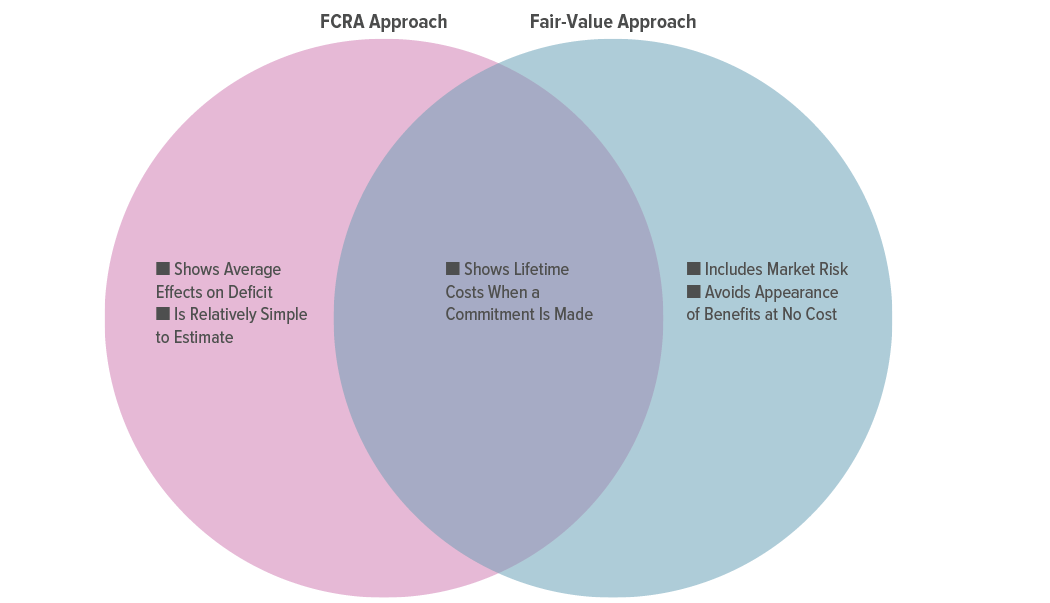
Like FCRA measures, fair value represents the cost today of programs that will result in future cash flows. Unlike those measures, fair value uses a more comprehensive measure of the risk of those programs by basing their estimated cost on how the private sector would value the cash flows of the loans or loan guarantees (see Figure 1). Fair-value budgeting also can be used to analyze other risky government activities—besides credit programs—such as insurance programs and retirement benefits.

Figure 1.

Advantages of an Accrual-Based System

Data source: Congressional Budget Office.

FCRA = Federal Credit Reform Act.

Fair-value budgeting takes into account the fact that financial assets tend to perform poorly when the economy is weak. At those times, borrowers default on their debt obligations more frequently, and amounts recovered from borrowers are smaller. Current and future generations bear the costs of the losses, which can result in higher taxes, lower spending, or greater debt. FCRA estimates only consider the effect of weak economic conditions based on their probability of occurring. Fair-value estimates place greater weight on those economic conditions, as resources tend to be scarce and particularly valuable during those more difficult times.

By valuing loans and loan guarantees using market prices or an estimation of those prices, the fair-value approach provides lawmakers with additional information about the cost of federal credit programs. The fair-value approach captures the risk that results from fluctuations in the overall economy—a risk to which the government is exposed in the same way as the private sector, even though the government can generally borrow money at a lower interest rate than private-market participants. But those lower Treasury rates do not reduce the cost to taxpayers of the market risk associated with federal credit programs. Treasury rates are relatively low because Treasury securities are backed by the government’s ability to raise taxes and reduce other spending. Nevertheless, when the government makes a risky loan to a borrower, it is effectively imposing that risk on the public. If the borrower defaults on the loan, the government’s debt is greater than it otherwise would have been, and the public is worse off.1

Pros and Cons of Each Approach

The FCRA and fair-value approaches to measuring costs have advantages and disadvantages, depending on the circumstances and purpose of their use. In some cases, the difference between costs estimated using the approaches is small, and in other cases it is larger. Some programs and activities face more market risk than others; for those programs, the FCRA approach indicates either greater savings or lower costs.

• To understand the likely effect of a policy on projected federal debt, FCRA is more useful than fair value because the cost measure under FCRA represents the average projected effect on the debt. When an estimate of the cost of a loan or loan guarantee is made, its actual cash flows are not known because the rate at which borrowers will default is uncertain. If the actual cash flows turn out to match those that are projected to occur, on average, the eventual effect on the debt will match the FCRA estimate.
• When policymakers are considering the costs of different forms of government assistance, fair-value estimates are more useful because FCRA estimates do not capture all the costs associated with loans and loan guarantees. If, for example, policymakers chose to support a private-sector activity, they could do so either by making loans to the affected individuals and businesses or by providing money through grants. The cost of the grants would simply be the same as the provided amount, but the cost of the loans would depend on the amount borrowers were likely to repay—and therefore could be much higher than projected if the economy was weak and borrowers defaulted on their loans at above-average rates. A fair-value estimate would incorporate the possibility of those additional defaults and thus would more completely measure the cost of the loans (relative to a FCRA estimate).
• FCRA estimates are more likely to produce the appearance of budgetary savings (in other words, show a negative cost) for activities that could be costly to government stakeholders. Fair-value estimates, by contrast, avoid the implication that the government can reduce the deficit just by making loans and guarantees at market rates (an implication that is often called a free lunch). In a competitive market, private investors charge interest and fees that fully offset the average cost of defaults and market risk. A FCRA estimate for a loan made at market prices would incorporate the interest and fees that a private investor would charge for market risk but not the cost of the market risk itself. As a result, under FCRA, a given loan or loan guarantee would appear less expensive when made by the federal government than if it was made by a private lender. The cost of market risk would be included in fair-value estimates, making estimates of the costs of loans and loan guarantees more comprehensive (and higher) using that measure.
• Fair-value estimates have some characteristics that can limit their usefulness. Even though both fair-value and FCRA estimates use discount rates that can vary over time, changes in the cost of market risk can make fair-value estimates more volatile. For that reason, they are more prone to uncertainty, particularly in a financial crisis when markets are not functioning well and transactions are disorderly. In addition, producing fair-value estimates is more complex and time-consuming than producing FCRA estimates (in part because it is difficult to measure the cost of market risk when it is unobservable), and communicating the basis for fair-value estimates to policymakers and the public is more challenging than communicating the basis for FCRA estimates, which is more straightforward.

Examples of the Approaches

The difference between costs measured using the FCRA and fair-value approaches can be seen through four examples of their application to various programs and activities.

• The Troubled Asset Relief Program (TARP), which by law is measured using the fair-value approach;
• Student loans, which by law are measured using the FCRA approach;
• Federal insurance, which is measured on a cash basis; and
• Investments in risky financial assets.

Those examples cover a wide range of government activities. In each case, the estimate of their costs would almost always be higher under fair value because that measure more comprehensively accounts for risk.

TARP

TARP was set up in 2008 to enable the Department of the Treasury to promote stability in financial markets through the purchase and guarantee of “troubled assets.” Its costs were required to be measured on a basis that was equivalent to fair value, meaning that they needed to include the market risk involved in having the government invest in banks, insurance companies, automobile companies, and other assets. CBO’s initial estimates for the Capital Purchase Program (CPP), in which TARP funds were invested in preferred shares of banks, showed that costs would be significant if measured using a fair-value approach, which would incorporate the cost of the risk associated with the banks’ failures and the Treasury’s loss of its investment; in contrast, the program would be expected to reduce deficits, on average, if its costs were measured using the FCRA approach.

The economy and housing market began to recover in late 2008 and early 2009 (soon after the initial cost estimates were published), and the CPP ultimately reduced federal budget deficits overall. That recovery was uncertain when the government took on the risk of the CPP’s investments, though—indeed, at that time, private-market participants required extraordinary compensation to invest in bank shares. Under FCRA, the government would have bought the assets at market prices and reported an instant profit, because the Treasury would have received a dividend yield on its preferred shares that exceeded its cost of borrowing and received warrants from the participating banks. The warrants, which gave the Treasury the right but not the obligation to purchase common stock at a favorable price, would have added to the income that the Treasury received from the dividends on the preferred stock. Although those terms more than offset the average cost of defaults, they would not have been sufficient for private investors to take on the same risk as the government, as reflected in the fair-value estimates at the time (which showed the investments increasing the deficit).

Even a fair-value analysis can miss important aspects of the impact of a policy in the midst of a crisis, because that analysis does not account for the budgetary effects of macroeconomic changes, which can be very significant in those situations (for details, see Box 1).

Student Loans

Higher limits on the amount of money that students could borrow for postsecondary education would result in more loans to students. That larger volume of loans would have a greater cost under the fair-value approach than under the FCRA approach because the cash flows of the student loan programs are subject to market risk: Former students tend to have lower income when the economy is performing poorly (because well-paying jobs are scarce), and the rate of defaults on student loans tends to be higher as well. A fair-value measure incorporating that market risk represents what the government would need to pay private entities to take on the cash flows from the loans. By contrast, a FCRA measure represents an amount of current cash spending that would have the same long-run effect on the debt as the student loans if defaults occurred at average rates.

Federal Insurance Programs

The federal budget typically measures the costs of programs on a cash basis and over a 10-year period. That period may be too short to accurately show some programs’ expected net effects—especially for programs that have long-term budgetary effects—which may cause timing-related distortions in their projected costs. That concern applies particularly to federal pension insurance that is supplied by the Pension Benefit Guaranty Corporation (a government corporation), because it may take more than 20 years to fully realize the costs of resolving or providing financial assistance to a distressed or terminated pension plan. By showing lifetime costs up front, present-value measures can avoid those distortions and allow for more meaningful comparisons of the costs of competing programs.

The present-value cost of federal insurance programs can be measured using the FCRA or fair-value approach. For federal insurance programs that face significant amounts of market risk (such as pension insurance), fair-value measures would result in more comprehensive (and much higher) estimates of their costs. For programs that have little market risk, such as crop insurance and flood insurance, the difference between fair-value and FCRA measures of their costs would be smaller. In those cases, using fair value would not make much difference and may not be worth the time and effort because FCRA is a close enough approximation to the more comprehensive fair-value measure of cost.

Investments in Risky Financial Assets

When estimates of average cash flows are used in the budget, the government’s purchase of risky financial assets at their market prices can appear to reduce deficits. Under the fair-value approach, those transactions would not affect the budget deficit.

When the National Railroad Retirement Investment Trust (NRRIT), a government-run trust fund covering railroad workers, started buying stocks and bonds in the early 2000s, a projection of the fund’s average cash flows would have shown savings, on net. Such a projection also would have given the impression that the improvement in average outcomes had no other consequences—in particular, it would not have accounted for the greater exposure of government stakeholders to market risk. CBO and the Office of Management and Budget (OMB) avoided that impression of a free lunch by projecting the earnings of the NRRIT’s investments using a Treasury rate of interest. That method reflected economic theory, which suggests that the difference between the average return on a risky asset and the interest rate on Treasury securities is equal to the cost of the risky asset’s additional risk.

That approach to the NRRIT’s investments is one precedent relevant to how CBO and OMB could view proposals to invest Social Security contributions in risky financial assets, either by investing Social Security trust funds in such assets or by incorporating individual accounts into the Social Security program. Although investing in the stock market would improve the projected balances in the Social Security trust funds or in private accounts, on average, it would also make those projected balances much more uncertain. Applying the same approach that was used for the NRRIT—that is, projecting earnings using Treasury rates regardless of what assets are held by the trust funds—would eliminate all of the added projected gains from investing in stocks.